Neural Networks, CNNs, RNNs, Transformers, and Beyond

This post is a very long introduction to various kinds of machine learning models and their ethical and societal implications. Jump to

• Neural Networks: The Foundation
  • Training
• Convolutional Neural Networks (CNNs)
  • Variants of CNNs
• Fundamentals of Language Processing
• Recurrent Neural Networks (RNNs)
  • Long Short-Term Memory (LSTMs)
• Transformers
  • Different Types of Transformers
• Generative Models
  • Generative Adversarial Networks (GANs)
  • Variational Autoencoders (VAEs)
  • Diffusion Models
• State Space Models (SSMs)
• Graph Neural Networks (GNN)
• Deep Reinforcement Learning
• Ethical and Societal Implications

Neural Networks: The Foundation

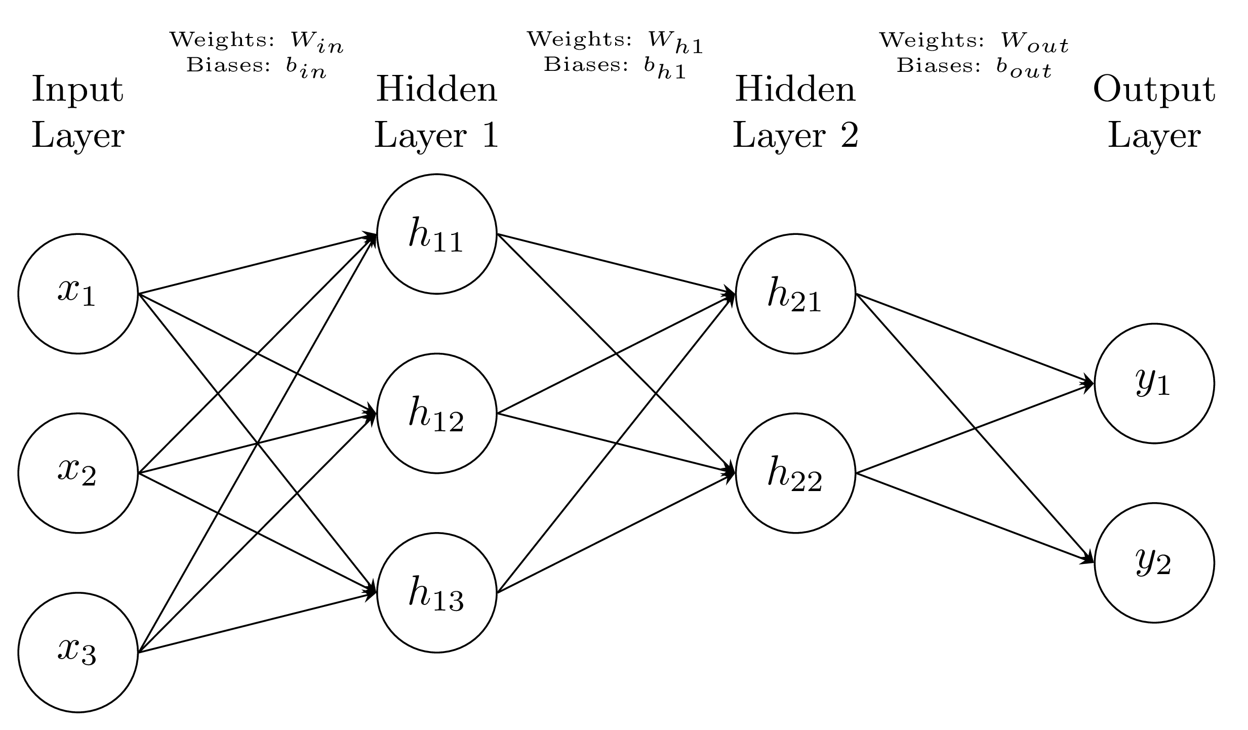
A neural network is a computational model inspired by the human brain. It consists of layers of interconnected neurons (or nodes), each performing a weighted summation followed by a non-linear activation function.

Mathematical Representation

Consider an input vector \(\mathbf{x}\in\mathbb{R}^n\), weights \(\mathbf{W}\in\mathbb{R}^{m\times n}\), biases \(\mathbf{b}\in\mathbb{R}^m\), and activation function \(f(\cdot)\). The output of a single layer is

\[\mathbf{h} = f(\mathbf{W}\mathbf{x} + \mathbf{b}).\]

Stacking these layers allows the network to learn hierarchical representations:

\[\mathbf{h}^{(k+1)} = f(\mathbf{W}^{(k)} \mathbf{h}^{(k)} + \mathbf{b}^{(k)})\]

The figure below illustrates this “stacking” process:

Training

It is now clear that training aims to obtain $\mathbf{W}$ and $\mathbf{b}$. Define a loss function, $L(\theta)$, to be minimized by adjusting $\mathbb{W}$ and $\mathbb{b}$, call them $\theta$. The optimizer achieves this by repeatedly calculating the gradient of the loss function, $\nabla_{\theta}L$, using backpropagation and updating the parameters via gradient descent. First, after a forward pass computes the network’s output and its resulting error or loss, the backpropagation algorithm performs a backward pass. During this pass, it efficiently calculates the gradient of the loss function, $\nabla_{\theta}L$, by applying the chain rule of calculus recursively from the final layer back to the first, determining how much each parameter contributed to the error. Finally, the gradient descent optimizer uses these calculated gradients to update all the network’s parameters, $\theta$, according to $\theta_{t+1} = \theta_t - \eta \nabla_{\theta}L(\theta_t)$, slightly adjusting them to minimize future error. To create sparsity, add a regularization penalty like the $\ell_1$ norm, $\lambda \sum |\theta_i|$, to the loss function, which actively forces many parameter values to become zero.

Theoretical Foundations

The capacity of neural networks to approximate any continuous function on a compact domain is guaranteed by the universal approximation theorem(s), stating that a neural network with at least one hidden layer and a non-linear activation function can approximate any continuous function to an arbitrary degree of accuracy (Cybenko, 1989; Hornik et al., 1989). People later proved that a network with a fixed, minimal width can be a universal approximator, provided it can have arbitrary depth (Lu et al., 2017; Kidger & Lyons, 2020). These theorems are purely existential, offering no guarantees on the efficiency of learning algorithms or the number of neurons required to achieve a prescribed approximation error.

Surprisingly, the loss surface of a large multilayer network is not fraught with poor local minima but is instead dominated by numerous saddle points and local minima whose loss values are qualitatively close to the global minimum (Choromanska et al., 2015). Counterintuitively, overparameterization can improve generalization, a behavior reconciled by double descent, which subsumes the classical bias-variance trade‐off into a unified framework where increasing capacity beyond interpolation lowers test error due to implicit regularization by the optimization algorithm (Belkin et al., 2019).

Practical Implementation

Modern deep learning hinges on flexible frameworks that abstract computational graphs, automatic differentiation, and hardware acceleration to streamline prototyping and large‐scale training. One important problem is the vanishing or exploding gradients problem, which arises in deep networks because backpropagation repeatedly multiplies gradients through each layer, causing the update signal to either shrink exponentially toward zero (vanishing), which prevents early layers from learning, or grow uncontrollably large (exploding), which makes the training process unstable. Initialization schemes like He initialization align weight variances with layer activations to mitigate this.

Batch normalization stabilizes activation distributions and accelerates deep convolutional training by explicitly normalizing layer inputs via batch‐wise mean and variance (enabling higher learning rates and less sensitivity to initialization) (Ioffe & Szegedy, 2015). Recently, researchers found that the dynamic tanh approach, which replaces all normalization layers in Transformers with a single learnable element-wise $\tanh(\alpha x)$, can further offer a practical, statistics-free alternative whenever batch or layer statistics are impractical or too costly (Zhu et al., 2025).

Adaptive optimizers such as Adam adjust per‐parameter learning rates based on estimates of first and second moments, offering robustness in sparse or noisy gradient scenarios and often outperforming vanilla SGD in practice (Kingma, 2014), overcoming the saddle point problem. Effective hyperparameter tuning—through systematic searches, Bayesian methods, or bandit algorithms—and rigorous experiment tracking (e.g., with TensorBoard or Weights & Biases) is critical for replicable state‐of‐the‐art results.

Empirical Understandings

Empirical scaling laws for language models demonstrate that cross‐entropy loss follows power‐law relationships with respect to model parameters, dataset size, and compute, allowing practitioners to predict performance gains and allocate resources optimally (Kaplan et al., 2020). The double descent phenomenon explains why enlarging model capacity can paradoxically reduce test error even after achieving zero training loss, unifying classical and modern generalization theories under one curve (Belkin et al., 2019). Moreover, the lottery ticket hypothesis reveals that within dense, randomly‐initialized networks lie sparse subnetworks (winning tickets) that, when trained in isolation, can match or exceed the accuracy of the full model, offering new directions for pruning and efficient inference (Frankle & Carbin, 2018).

Convolutional Neural Networks (CNNs)

CNNs are specialized for data with spatial structure, like images. Instead of fully connected layers, they use convolutional layers to extract local patterns, such as edges in images (corresponding to shapes in the image). Multiple layers are involved in this process (LeCun et al., 2002).

Mathematical Representation

A convolution operation involves a filter (or kernel) \(\mathbf{K} \in \mathbb{R}^{k \times k}\) sliding over the input \(\mathbf{X} \in \mathbb{R}^{n \times n}\):

\[(\mathbf{X} * \mathbf{K})_{ij} = \sum_{p=0}^{k-1}\sum_{q=0}^{k-1} \mathbf{X}_{i+p, j+q} \mathbf{K}_{p, q}\]

The output is called a feature map. The figure below illustrates this process:

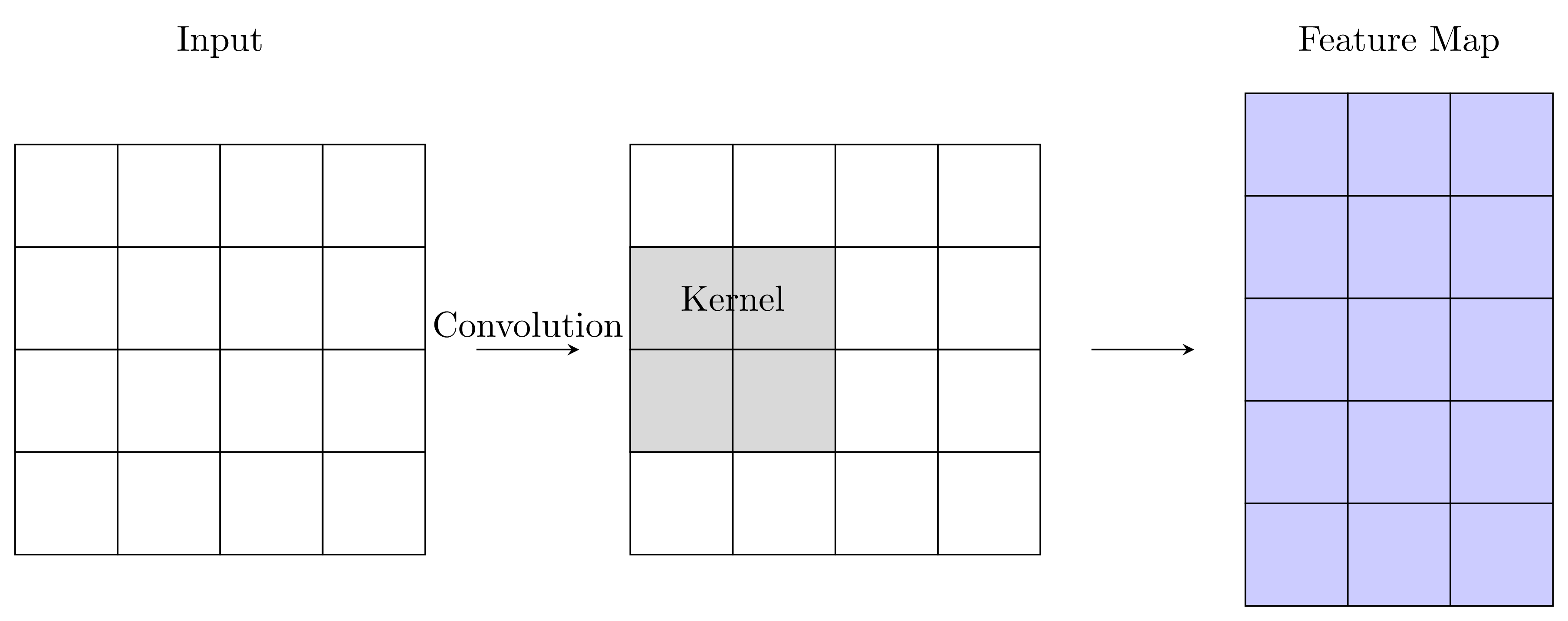
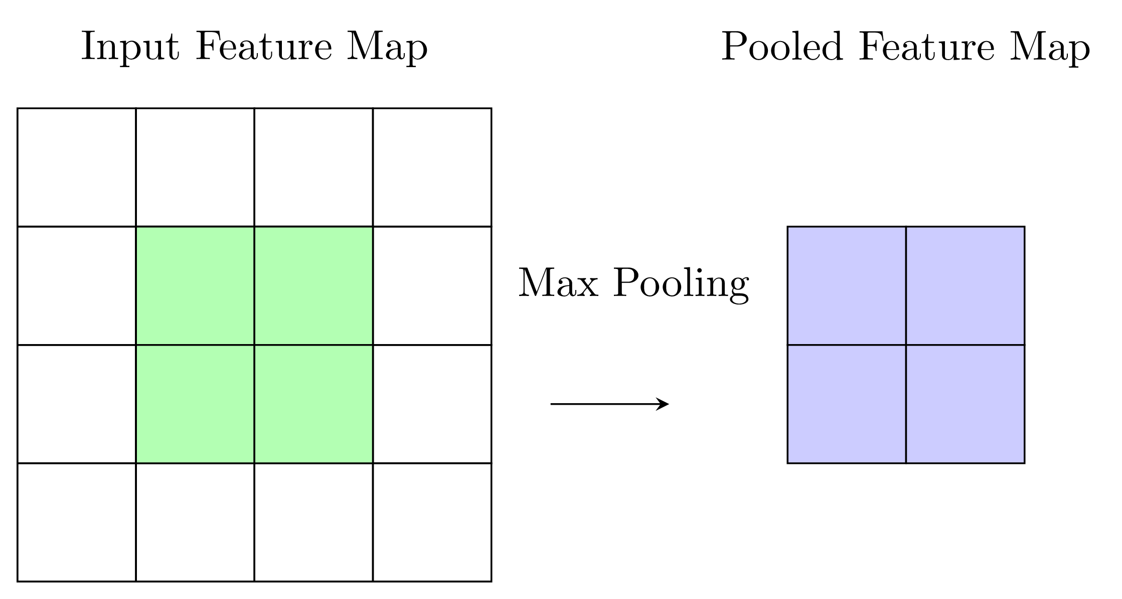
The starting point of this illustration demonstrates that CNNs are naturally useful for images or videos — we can view each pixel as a single cell of the input above. Pooling layers (e.g., max pooling) then downsample these feature maps, reducing dimensionality:

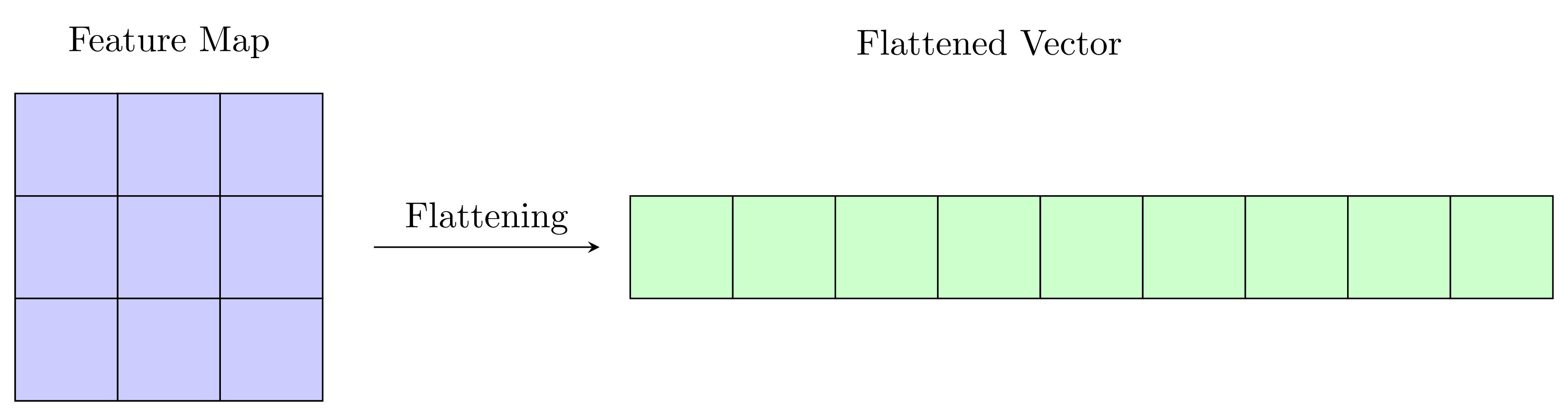
The flattening process converts the feature maps in \(\mathbb{R}^{H \times W \times D}\) to a 1-D vector (e.g., in \(\mathbb{R}^{K}\)):

Lastly, a fully connected layer connects the vector to the output layer,

\[\mathbf{h}^{(k+1)} = f(\mathbf{W}^{(k)} \mathbf{h}^{(k)} + \mathbf{b}^{(k)}).\]

CNNs apply the same filter across the input and focus on local patches. Layers capture increasingly complex features (e.g., edges → textures → objects).

Foundations

The convolution operation embeds a translation equivariance prior by sharing the same kernel across spatial locations, drastically reducing the number of free parameters compared to fully connected layers and enabling the detection of local patterns regardless of their position in the image. Beyond parameter efficiency, the universal approximation properties of deep convolutional architectures stem from their ability to hierarchically compose simple linear filters and pointwise nonlinearities to approximate increasingly complex functions, a concept formalized in early work on multi-layer perceptrons and extended to convolutional settings (LeCun et al., 2002). The scattering transform framework interprets CNNs as cascades of wavelet convolutions and modulus operations, proving Lipschitz stability to deformations—a proxy for robustness to small geometric perturbations—while still capturing discriminative signal variations (i.e., higher-order interactions) (Mallat, 2012). Theoretical analyses have also shown a surprising result, where modern deep nets, including CNN, have enough capacity to memorize random labels (i.e., achieve zero training error on noise) with no explicit regularization (Zhang et al., 2016).

Empirical studies of feature transferability reveal that early convolutional layers learn general patterns such as edge and texture detectors, while deeper layers capture task-specific semantics; transferring features from mid-level layers provides the best balance between generality and specificity for new tasks (Yosinski et al., 2014).

Variants of CNNs

Early landmark models such as AlexNet (Krizhevsky et al., 2012) train on ImageNet (Deng et al., 2009) demonstrated that deep convolutional architectures trained on large-scale datasets with GPUs could achieve dramatic improvements in object recognition, introducing ReLU activations ($f(x)=\max(0,x)$), data augmentation techniques (in-memory reflections and intensity alternation), and dropout (temporarily randomly deactivating neurons) as a regularizer to mitigate co-adaptation of neurons. Subsequent architectures explored the impact of depth and filter granularity: VGGNets (Simonyan & Zisserman, 2014) showed that stacking small $3 \times 3$ convolutions to reach depths of 16–19 layers yields improved representational power and transferability across tasks, while Inception modules factorized convolutions into multiple filter sizes to better utilize computational resources and capture multi-scale context (Szegedy et al., 2015). The introduction of residual connections overcame optimization difficulties in very deep models by reformulating each layer as a residual mapping, enabling stable training of networks exceeding 100 layers and pushing error rates below 4% on ImageNet (He et al., 2016). More recently, compound scaling methods systematically balance depth, width, and resolution by a single coefficient, resulting in EfficientNet families that deliver superior accuracy-efficiency trade-offs and generalize effectively across transfer-learning benchmarks (Tan & Le, 2019; Tan & Le, 2021).

Fundamentals of Language Processing

Before introducing sequential models, let’s first see how we can represent texts numerically, which is not as straightforward as image representation (pixel grids). Remember models understand numbers.

Before embedding, raw text is segmented into subword tokens via algorithms such as Byte-Pair Encoding, which greedily merges the most frequent character pairs to yield a fixed-size vocabulary that balances morphological expressiveness and open-vocabulary coverage (Sennrich et al., 2015).

Byte-Pair Encoding (BPE) Example

1. Initial State: Start with a corpus (e.g., low lower lowest) and break words into characters plus an end-of-word marker (l o w </w>). The initial vocabulary is just these characters.

2. Greedy Merging: Iteratively find the most frequent adjacent pair and merge it into a new token.
   • Step 1: The pair l o is most frequent. Merge it to create the token lo. The vocabulary is now [l, o, w, ..., lo].
   • Step 2: The pair lo w becomes the most frequent. Merge it to create low. The vocabulary is now [l, o, w, ..., lo, low].
3. Result: This continues until a target vocabulary size is reached.
   • Morphological Expressiveness: A known word like lowest is tokenized into meaningful parts, like [low, est].
   • Open-Vocabulary Coverage: An unknown word like slower can still be represented by falling back to known subwords and characters, like [s, l, o, w, er].

Each token $t_i$ is then represented as a one-hot vector $x_i\in\mathbb{R}^{|V|}$, where $|V|$ is the vocabulary size, and mapped into a dense embedding $e_i = E^\top x_i$ using an embedding matrix $E\in\mathbb{R}^{|V|\times d}$, capturing lexical semantics in a continuous space (Mikolov et al., 2013). Subword tokenization is the most efficient and manageable tokenization method thus far, as opposed to character and word tokenizations. Transformers inject positional information lost by parallel processing, a fixed sinusoidal encoding $P\in\mathbb{R}^{n\times d}$ is added, where

\[P_{i,2k} = \sin\!\bigl(i/10000^{2k/d}\bigr),\quad P_{i,2k+1} = \cos\!\bigl(i/10000^{2k/d}\bigr),\]

yielding $Z = [e_1; \dots; e_n] + P$ as the input to subsequent layers. The famous attention mechanism then comes into play (Vaswani et al., 2017).

For ideographic languages such as Chinese and Japanese, the default approach treats each character as a base token, but recent sub-character methods (Si et al., 2023; Nguyen et al., 2017) first transliterate characters into sequences of glyph strokes or phonetic radicals before applying BPE, allowing models to inject rich visual and pronunciation.

Recurrent Neural Networks (RNNs)

RNNs (Elman, 1990) excel at processing sequential data, such as time series or text. They maintain a memory of previous inputs via a hidden state, allowing them to model temporal dependencies.

Mathematical Representation

RNNs process data sequentially. At each time step \(t\), an input \(\mathbf{x}_t\) is provided. The sequence of inputs can be represented as \(\mathbf{x}_1\), \(\mathbf{x}_2\), up to \(\mathbf{x}_T\), where \(T\) is the total number of time steps. RNNs maintain a hidden state, \(\mathbf{h}_t\), acting as the network’s memory, updated at each time step based on the current input and the previous hidden state.

Given input \(\mathbf{x}_t\), hidden state \(\mathbf{h}_t\), and weights \(\mathbf{W}_{xh}\), \(\mathbf{W}_{hh}\), the hidden state is updated as

\[\mathbf{h}_t = f(\mathbf{W}_{xh} \mathbf{x}_t + \mathbf{W}_{hh} \mathbf{h}_{t-1} + \mathbf{b}).\]

The output \(\mathbf{y}_t\) is computed as:

\[\mathbf{y}_t = g(\mathbf{W}_{hy} \mathbf{h}_t + \mathbf{c}).\]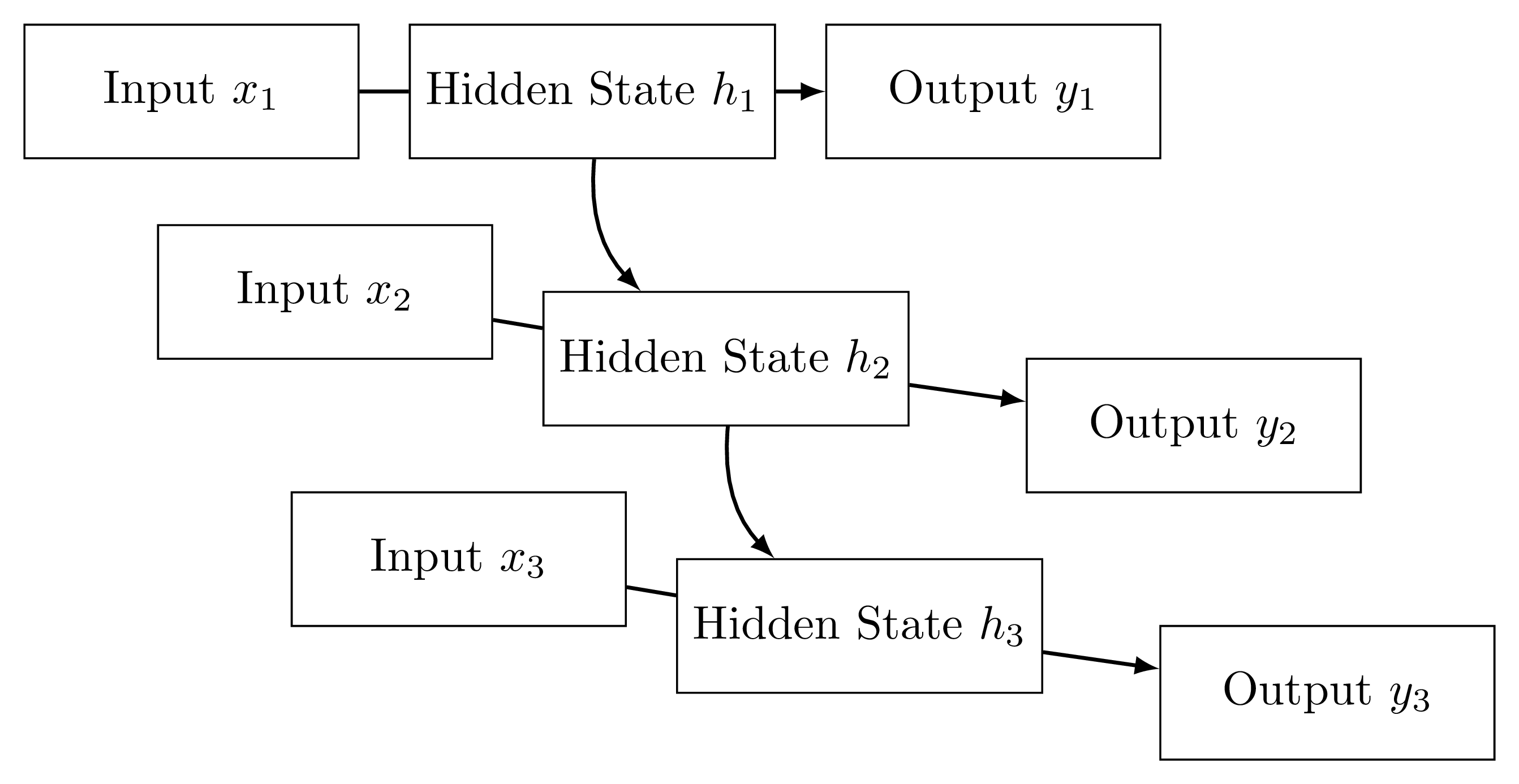

Limitations and Development

RNNs suffer inherently from gradients that either vanish or explode exponentially with depth in time when signals are propagated over many time steps, making naive RNNs impractical for long‐term dependencies (Hochreiter, 1998; Bengio et al., 1994; Pascanu et al., 2013). Long Short-Term Memory cells (Hochreiter & Schmidhuber, 1997) mitigate this by embedding gating units that learn to preserve information in a constant‐error carousel, thereby enabling the modeling of arbitrarily distant dependencies without gradient collapse (Hochreiter & Schmidhuber, 1997). Subsequent work on Recurrent Highway Networks (Zilly et al., 2017) extended depth within each time step, applying gated residual connections to achieve deep transition functions that retain the LSTM’s long‐range memory while improving representational capacity. Alternative approaches constrain the recurrent weight matrix to be orthogonal or unitary, ensuring gradient norms remain constant and thus preserving signal propagation over arbitrary horizons without numerical instability (Mhammedi et al., 2017; Arjovsky et al., 2016). Further, continuous‐time formulations like Neural ODEs reimagine recurrence as the discretization of a differential equation, offering a unified view of depth and time and opening the door to adaptive computation and memory allocation strategies (Chen et al., 2018).

Long Short-Term Memory (LSTMs)

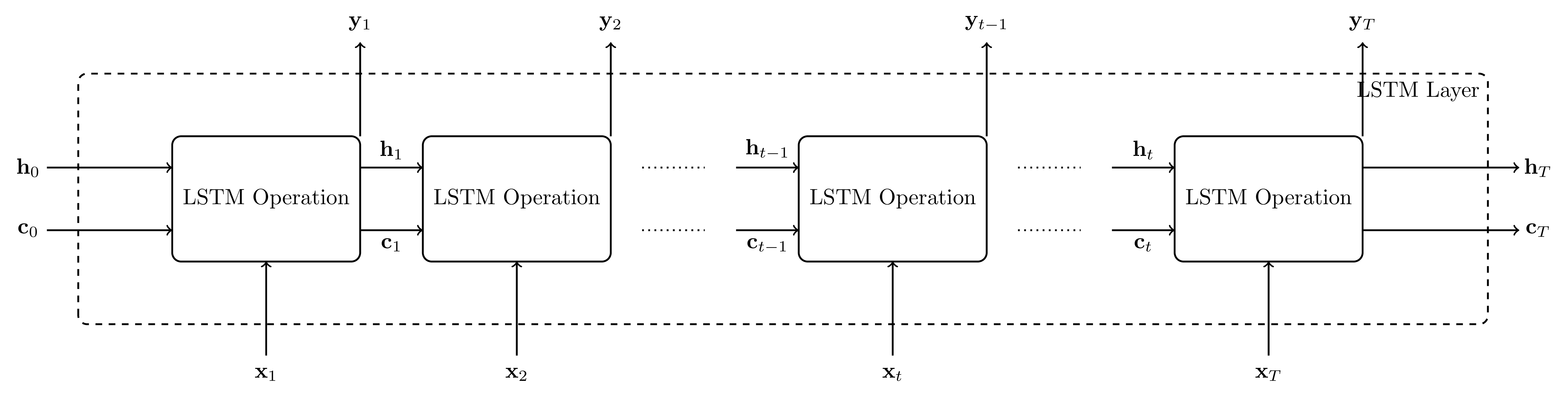
LSTMs (Hochreiter & Schmidhuber, 1997) improve on standard RNNs by controlling the flow of information, using gates to selectively remember, forget, or output information, allowing the network to retain long-term dependencies. The graph below illustrates this sequential structure, which is structurally similar to RNNs:

Mathematical Representation

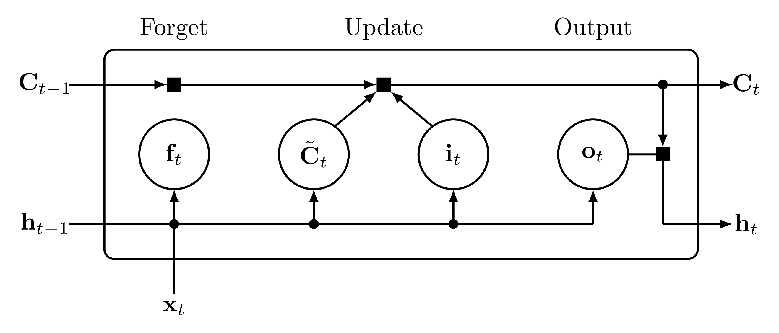
Here, \(\sigma(\cdot)\) is the sigmoid activation, \(\tanh(\cdot)\) is the hyperbolic tangent, and \(\odot\) represents element-wise multiplication. At each time step \(t\), the LSTM maintains long-term memory called a cell state (\(\mathbf{C}_t\)) and short-term memory called a hidden state (\(\mathbf{h}_t\)). They also introduce 3 types of gates:

1. Forget Gate (\(\mathbf{f}_t\)): Decides which information to discard from the cell state:

   \[\mathbf{f}_t = \sigma(\mathbf{W}_f \mathbf{x}_t + \mathbf{U}_f \mathbf{h}_{t-1} + \mathbf{b}_f).\]

2. Input Gate (\(\mathbf{i}_t\)): Decides which new information to add to the cell state:

   \[\mathbf{i}_t = \sigma(\mathbf{W}_i \mathbf{x}_t + \mathbf{U}_i \mathbf{h}_{t-1} + \mathbf{b}_i).\]

   Candidate Cell State: The candidate cell state (\(\tilde{\mathbf{C}}_t\)) is computed as:

   \[\tilde{\mathbf{C}}_t = \tanh(\mathbf{W}_C \mathbf{x}_t + \mathbf{U}_C \mathbf{h}_{t-1} + \mathbf{b}_C).\]

3. Output Gate (\(\mathbf{o}_t\)): Decides the output based on the hidden state and cell state:

   \[\mathbf{o}_t = \sigma(\mathbf{W}_o \mathbf{x}_t + \mathbf{U}_o \mathbf{h}_{t-1} + \mathbf{b}_o)\]

Updating the States

1. Cell State Update:

   \[\mathbf{C}_t = \mathbf{f}_t \odot \mathbf{C}_{t-1} + \mathbf{i}_t \odot \tilde{\mathbf{C}}_t\]

   The forget gate decides what to discard, and the input gate decides what to add.

2. Hidden State Update:

   \[\mathbf{h}_t = \mathbf{o}_t \odot \tanh(\mathbf{C}_t)\]

The graph below illustrates this updating process:

Practical Implementation

Training recurrent models requires balancing sequence length, computational budget, and numerical stability; truncated backpropagation through time (TBPTT) (Williams & Zipser, 1989) limits gradient propagation to manageable windows while approximating full‐sequence gradients, and gradient clipping (Pascanu et al., 2013) prevents rare but disastrous exploding updates. Layer and weight regularization techniques—such as DropConnect in the AWD‐LSTM architecture (Merity et al., 2017) and variational dropout (Kingma et al., 2015)—act directly on recurrent weights and activations to reduce overfitting in language modeling tasks, allowing smaller datasets to yield robust sequence predictors. Modern deep learning frameworks provide native implementations of these gating and optimization schemes, and tools like mixed‐precision training (Micikevicius et al., 2017) and distributed sequence parallelism (Merity et al., 2017; Korthikanti et al., 2023; Jacobs et al., 2023) make it feasible to train very deep or very long‐sequence models on GPUs and TPUs with reproducible results (Merity et al., 2017).

Empirical Understandings

Empirical benchmarks on language modeling datasets reveal that carefully regularized LSTMs such as AWD‐LSTM (Merity et al., 2017) achieve state‐of‐the‐art perplexities on Penn Treebank (Marcus et al., 1993) and WikiText‐2 (Merity et al., 2016), demonstrating the continued relevance of gated recurrence for moderate‐scale tasks. However, scaling studies show that beyond a certain compute and data threshold, self‐attention architectures outperform traditional RNNs in both speed and quality (Kaplan et al., 2020), prompting hybrid approaches that inject attention mechanisms into LSTM backbones (Bahdanau et al., 2014) or employ Neural ODE layers for continuous modeling (Chen et al., 2018). Ablation experiments on gating variants and transition depths indicate that deeper recurrent transitions and highway connections yield diminishing returns beyond a handful of layers per step, suggesting that future gains will depend on novel memory‐access patterns or adaptive computation time mechanisms (Desbouvries et al., 2023; Zilly et al., 2017). As attention‐first models (introduced next section) continue to dominate, the most promising directions revive recurrence through continuous dynamics, orthogonal memory networks, and differentiable neural computers that combine the best of gating, memory, and attention in a unified framework.

Transformers

In the transformer (Vaswani et al., 2017), we represent an input sequence of $n$ tokens by their embeddings $X\in\mathbb{R}^{n\times d}$ and compute three projections—queries $Q=XW^Q$, keys $K=XW^K$, and values $V=XW^V$—each in $\mathbb{R}^{n\times d_k}$. Self‐attention is then given by

\[\mathrm{Attention}(Q,K,V)=\mathrm{softmax}\bigl(QK^{\!\top}/\sqrt{d_k}\bigr)\,V\,.\]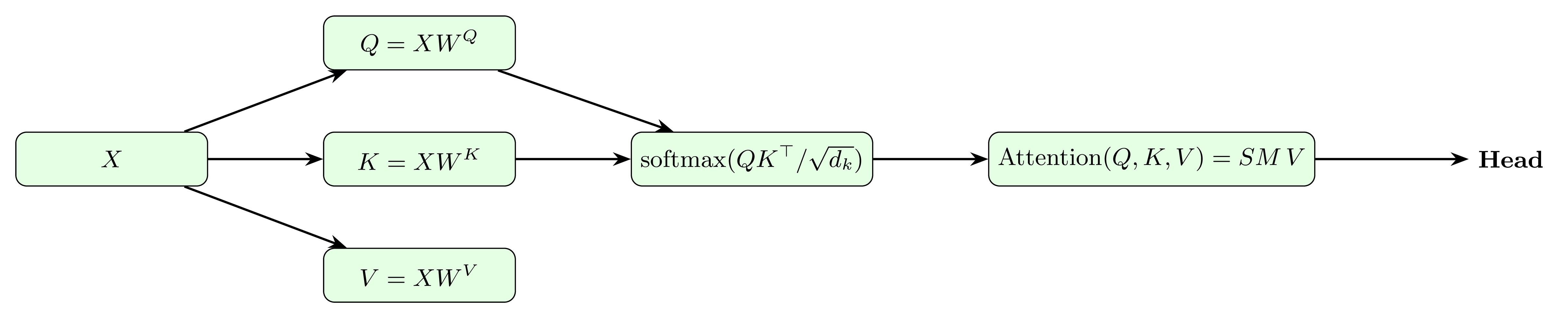

Multi‐head attention runs this in parallel for $h$ heads and concatenates the results:

\[\mathrm{MultiHead}(X)=\mathrm{Concat}\bigl(\mathrm{head}_1,\dots,\mathrm{head}_h\bigr)\,W^O,\quad \mathrm{head}_i=\mathrm{Attention}(XW^Q_i,XW^K_i,XW^V_i).\]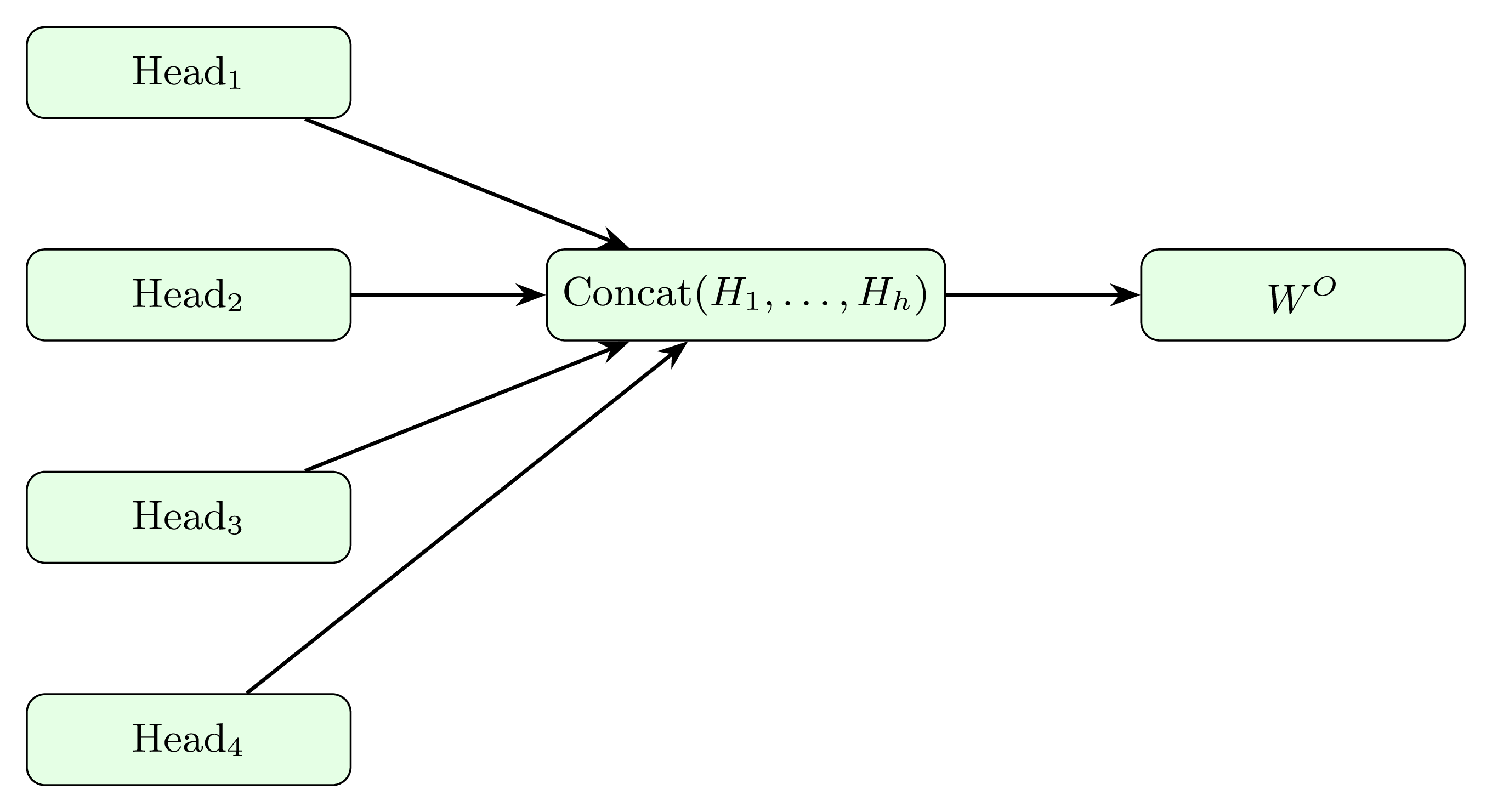

Each transformer layer applies a residual connection plus layer normalization, $\tilde X=\mathrm{LayerNorm}\bigl(X+\mathrm{MultiHead}(X)\bigr)$, followed by a position‐wise feed‐forward network

\[\mathrm{FFN}(\tilde X)=\sigma(\tilde XW_1+b_1)\,W_2+b_2\]

and another residual‐norm step $\mathrm{LayerNorm}\bigl(\tilde X+\mathrm{FFN}(\tilde X)\bigr)$. Stacking $L$ such layers yields the final contextual representations used for downstream prediction.

Different Types of Transformers

Beyond the canonical vanilla Transformer, nearly every variant introduces one or more mathematical tweaks to attention, embeddings, or the layer‐stacking strategy. A common class of modifications concerns positional information, via learned absolute embeddings (BERT (Devlin et al., 2019), GPT-2/3 (Radford et al., 2019; Brown et al., 2020), RoBERTa (Liu et al., 2019)), relative position biases (Transformer-XL (Dai et al., 2019), T5 (Raffel et al., 2020), DeBERTa (He et al., 2020)), or rotary position embeddings (RoFormer (Su et al., 2024), GPT-NeoX (Black et al., 2022)). In the original model, we add fixed sinusoidal encodings $P\in\mathbb{R}^{n\times d}$ so that the input to layer 1 is $X+P$. Later work replaces these with learned embeddings $P_\theta$, relative position biases $B_{ij}$, so that attention becomes

\[\mathrm{softmax}\bigl((QK^\top + B)/\sqrt{d_k}\bigr)\,V,\]

where $B\in\mathbb{R}^{n\times n}$ depends only on $i-j$, or even rotary embeddings that apply a learnable $2 \times 2$ rotation to each pair of dimensions in $Q$ and $K$ before dot‐product. Such tweaks allow the model to better generalize to sequences longer than it saw in training, or to bias attention toward nearby tokens without explicit masking.

Another rich vein of innovation is efficient or specialized attention. For truly long sequences, full $n\times n$ attention is quadratic in cost; sparse‐attention variants insert a structured mask $M$ so

\[\mathrm{Attention}(Q,K,V)=\mathrm{softmax}\bigl((QK^\top + M)/\sqrt{d_k}\bigr)V,\]

where $M_{ij}=-\infty$ for disallowed pairs (e.g. sliding windows in Longformer (Beltagy et al., 2020) or random/global tokens in BigBird (Zaheer et al., 2020)). Low‐rank or kernelized methods approximate

\[\mathrm{softmax}(QK^\top)\approx \phi(Q)\,\phi(K)^\top\]

via feature maps $\phi$, yielding linear time (Performer (Choromanski et al., 2020)). Other approaches project keys and values to a lower dimension: Linformer (Wang et al., 2020) posits learnable $E\in\mathbb{R}^{n\times k}$, $F\in\mathbb{R}^{n\times k}$ so that $K’=E^\top K$, $V’=F^\top V$, reducing attention to $\mathrm{softmax}(QK’^\top)V’$. Finally, mixtures‐of‐experts (Switch Transformers (Fedus et al., 2022)) replace each feed‐forward block with a routing mechanism $G(x)$ that selects among $m$ experts, so

\[\mathrm{MoE}(x) = \sum_{e=1}^m G_e(x)\bigl(W_2^{(e)}\,\sigma(W_1^{(e)}x)\bigr),\]

trading depth for conditional computation. Other architectures include GShard (Lepikhin et al., 2020) and GLaM (Du et al., 2022).

Together, these mathematical tweaks—positional biases, sparse or low‐rank attention, kernel approximations, adaptive-depth recurrence (Universal Transformer (Dehghani et al., 2018)), and conditional computation—form a rich taxonomy under the transformer umbrella, each tailored to specific tasks, modalities, or resource constraints.

Theoretical Understandings

A Transformer layer computes scaled dot-product attention, where queries, keys, and values are linear projections of the same input; the resulting attention matrix is then normalized by $\sqrt{d_k}$ to maintain gradient stability, and softmaxed to produce a distribution over positions (Vaswani et al., 2017). Multi-head attention extends this by learning multiple sets of projections, allowing the model to jointly attend to information from different representation subspaces at distinct positions, which empirically enhances expressivity and enables parallel processing of dependencies. Formal analysis reveals that self-attention matrices can approximate arbitrary sparse matrices—thus capturing selective interactions among tokens—provided sufficient hidden dimensionality, granting Transformers a universal approximation property for sequence-to-sequence functions (Likhosherstov et al., 2021). Positional encodings—either fixed sinusoidal functions or learned embeddings—inject order information lost by the permutation-invariant attention mechanism, allowing the network to distinguish between positions in a sequence while preserving the ability to generalize to longer sequences than seen during training. Recent theoretical work also explores linearized and sparse variants that reduce the quadratic complexity of full attention to linear or near-linear bounds, trading off exactness for scalability without sacrificing universal expressivity in the limit (Child et al., 2019; Choromanski et al., 2020).

Practical Implementation

Effective Transformer training hinges on stabilized optimization. The AdamW (Loshchilov & Hutter, 2017) optimizer decouples weight decay from gradient updates, mitigating the tendency of adaptive methods to over-regularize while preserving the fast convergence of Adam; coupled with a linear warmup schedule for the learning rate (often over the first 10% of training steps), it prevents instability caused by large initial updates (Kosson et al., 2024). Gradient clipping (Pascanu et al., 2013) is commonly employed to bound the norm of gradients, curtailing occasional spikes during backpropagation that could derail learning, especially in deep or high-capacity models. Frameworks such as the Hugging Face Transformers library provide modular building blocks—pretrained checkpoints, tokenizer classes, and optimized training loops—enabling researchers and practitioners to experiment with architectures like BERT, GPT, T5, and beyond using both PyTorch and TensorFlow backends with minimal boilerplate. Mixed-precision training (via NVIDIA’s Apex or native AMP) significantly reduces memory usage and increases throughput by storing activations and performing many computations in a 16-bit floating-point format; to maintain numerical stability, a 32-bit master copy of the weights is used for accumulating gradients, a process that necessitates dynamic loss scaling to prevent underflow of small gradient values. Recent adapter-based fine-tuning methods such as LoRA (Hu et al., 2022) inject low-rank parameter updates into attention layers, slashing the number of trainable parameters for efficient domain adaptation without full-model retraining. Additionally, in-context learning allows large-scale Transformers to perform novel tasks by conditioning solely on a handful of demonstration examples in the input prompt, without any gradient updates to model parameters, a meta-learning capability that emerges only at sufficient model scale and is predictive of downstream few-shot performance (Brown et al., 2020).

Empirical Understandings

Empirical scaling laws for Transformers reveal that cross-entropy loss on language tasks follows a power-law decay as a function of model parameters, dataset size, and compute budget, enabling precise forecasts of performance improvements for scale investments (Kaplan et al., 2020). At extreme scales, emergent capabilities—such as few-shot in-context learning (Brown et al., 2020), chain-of-thought reasoning (Wei et al., 2022), and compositional generalization (Anil et al., 2022)—materialize abruptly and unpredictably, indicating qualitative shifts in model behavior that defy simple extrapolation from smaller models (Wei et al., 2022). Benchmarks comparing encoder-only models (e.g., BERT), decoder-only models (e.g., GPT), and encoder-decoder models (e.g., T5) demonstrate trade-offs between understanding and generation: encoder-only excels on classification and extraction tasks, decoder-only leads on open-ended generation, and encoder-decoder offers strong performance in sequence transduction. Fine-tuning studies show that the highest layers capture task-specific features while mid-layers encode transferable linguistic abstractions, guiding strategies for parameter freezing or adapter insertion during domain adaptation (Jurafsky & Martin, 2025). As attention-driven models continue to dominate, the frontier now lies in integrating external memory (Graves et al., 2014), adaptive computation time, and hybrid architectures that marry recurrence, attention, and continuous-depth dynamics to push the envelope of sequence modeling further (Israel et al., 2025).

Generative Models

Generative modeling is one very important field in current applications and it encompasses a variety of approaches that trade off sample quality, training stability, and computational cost.

Generative Adversarial Networks (GANs)

A GAN consists of two neural networks—$G$ generates candidate samples from random noise, and $D$ discriminates between real and generated data—trained in a minimax game that converges when $G$ reproduces the true data distribution and $D$ cannot distinguish samples (Goodfellow et al., 2014). The core objective

\[\min_G \max_D \;V(D,G) =\mathbb{E}_{x\sim p_{\text{data}}}[\log D(x)] +\mathbb{E}_{z\sim p_z}[\log(1 - D(G(z)))]\]

encodes a zero-sum game where $D$ seeks to maximize its classification accuracy while $G$ seeks to fool $D$. Intuitively, this adversarial setup avoids explicitly defining a distance metric between distributions; instead, $D$ implicitly shapes $G$’s loss.

GANs are favored when high-resolution, perceptually realistic samples are required—image synthesis, style transfer (e.g., pix2pix (Isola et al., 2017)), and data augmentation in medical imaging. However, training dynamics can oscillate or diverge, and GANs commonly suffer from mode collapse, where $G$ outputs limited variations, undermining data diversity (Kossale et al., 2022). Techniques like Wasserstein GANs (Arjovsky et al., 2017), two-time-scale updates (Heusel et al., 2017), and minibatch discrimination (Salimans et al., 2016) partially mitigate these failures, but stable convergence remains a challenge.

Variational Autoencoders (VAEs)

VAEs frame generative modeling as approximate inference in a probabilistic graphical model (Kingma et al., 2013). An encoder network parameterizes a variational posterior $q_\phi(z\mid x)$ over latent $z$, and a decoder network defines $p_\theta(x\mid z)$. Training maximizes the evidence lower bound,

\[\mathcal{L}_{\theta,\phi}(x) =\mathbb{E}_{z\sim q_\phi(z\mid x)}[\log p_\theta(x\mid z)] -\mathrm{KL}\bigl(q_\phi(z\mid x)||p(z)\bigr),\]

balancing reconstruction fidelity against a Kullback–Leibler penalty that regularizes $q_\phi$ toward the prior $p(z)=\mathcal{N}(0,I)$. The reparameterization trick—expressing $z=E_\phi(x)+\sigma_\phi(x)!\odot!\epsilon$ with $\epsilon\sim\mathcal{N}(0,I)$—enables gradient descent.

VAEs excel in learning smooth, disentangled latent spaces for downstream tasks like interpolation, anomaly detection, and semi-supervised classification. They train reliably via maximum likelihood principles but often yield blurry outputs due to pixel-wise losses and can collapse the posterior to the prior (posterior collapse), losing latent expressivity (Wang et al., 2021). Intuitively, one can imagine this as a librarian giving up on complex filing systems and simply dumping every single book, regardless of what it is, directly into the central pile. Remedies include KL annealing (Bowman et al., 2015; Fu et al., 2019), $\beta$-VAEs (Higgins et al., 2017), and alternative divergences (Davidson et al., 2018).

Diffusion Models

Diffusion models cast generation as the learned reversal of a gradual, data-corrupting noising process (Sohl-Dickstein et al., 2015; Ho et al., 2020). This forward process is defined as a Markov chain that systematically adds Gaussian noise to the data over successive steps:

\[q(x_t\mid x_{t-1})=\mathcal{N}\bigl(x_t;\sqrt{1-\beta_t}\,x_{t-1},\;\beta_tI\bigr)\]

To generate new samples, a neural network—often a U-Net—is trained to learn the reverse “denoising” process, $p_\theta(x_{t-1}\mid x_t)$. The network is optimized by minimizing a variational upper bound on the negative log-likelihood, which trains it to reconstruct the data by incrementally removing the noise step by step.

By sidestepping adversarial objectives, diffusion models offer stable training and have achieved superior fidelity in image and audio synthesis—powering DALL-E 2 (Ramesh et al., 2022), and Stable Diffusion (Rombach et al., 2022)—while supporting inpainting, super-resolution, and conditioned generation. Their main limitation is inference cost: thousands of sequential denoising steps lead to slow sampling and high compute demands, motivating research on accelerated samplers and trading off steps for quality.

State Space Models (SSMs)

State space models formalize sequential data by positing an unobserved (latent) state $x_t\in\mathbb{R}^n$ that evolves linearly under additive Gaussian noise and generates observations $y_t\in\mathbb{R}^m$ through another linear mapping. In the canonical form,

\[x_t = A\,x_{t-1} + B\,u_t + w_t,\quad w_t\sim\mathcal N(0,Q),\quad y_t = C\,x_t + D\,u_t + v_t,\quad v_t\sim\mathcal N(0,R),\]

where $u_t$ denotes known inputs, and $Q,R$ are covariance matrices governing process and measurement noise (Kalman, 1960; Kalman, 1963; Durbin & Koopman, 2012).

Intuitively, the latent state $x_t$ captures the system’s memory and structure, while Bayesian filtering algorithms (e.g., the Kalman filter) recursively update the posterior $\mathbb P(x_t\mid y_{1:t})$ as new data arrive. The Kalman filter computes the minimum-variance estimate of the latent state via a predict–update cycle:

\[\hat x_{t|t-1}=A\hat x_{t-1|t-1}+B u_t,\quad P_{t|t-1}=A P_{t-1|t-1}A^\top+Q,\] \[K_t=P_{t|t-1}C^\top\bigl(CP_{t|t-1}C^\top+R\bigr)^{-1},\quad \hat x_{t|t}=\hat x_{t|t-1}+K_t\,(y_t-C\hat x_{t|t-1}),\quad P_{t|t}=(I-K_tC)\,P_{t|t-1}.\]

It yields the optimal minimum mean-square error estimate by minimizing $\mathbb{E}||x_t-\hat{x}_{t\mid t}||^2$ under Gaussian noise assumptions. When exact Gaussian updates become intractable—due to nonlinearity or high dimensionality—sequential Monte Carlo and MCMC methods provide flexible approximate inference.

These models are prized for handling noisy, partially observed time series: they naturally accommodate measurement error, cope with missing data, and decompose signals into interpretable components such as trend and seasonality. The linear Gaussian assumption, however, can fail when dynamics are strongly nonlinear or noise is non-Gaussian. The extended Kalman filter may diverge under severe nonlinearity, and even unscented variants can underperform if noise covariances are misspecified. More critically, simple SSMs can exhibit biased or imprecise parameter estimates when measurement error dominates true signal variance (Julier & Uhlmann, 2004; Auger-Méthé et al., 2016).

In practice, state space models underpin econometric forecasting and structural time series analysis (Harvey, 1990), speech recognition via continuous-emission HMMs (Rabiner, 2002), robotic localization and SLAM through probabilistic state estimation, and modern deep latent-variable learning such as deep Kalman filters for counterfactual inference in health care and vision (Krishnan et al., 2015). Recent advances in Gaussian process state-space models and fully variational inference further extend classical SSMs to nonparametric, high-dimensional settings (Fan et al., 2023; Särkkä & Svensson, 2023).

Graph Neural Networks (GNNs)

GNNs generalize deep neural networks to graph-structured data by iteratively aggregating information from each node’s local neighbourhood. Formally, a $k$-th layer representation of node $v$ is given by

\[h_v^{(k)} = \text{update}^{(k)}\bigl(h_v^{(k-1)},\;\text{aggregate}^{(k)}\{\,(h_u^{(k-1)},e_{uv}):u\in\mathcal{N}(v)\}\bigr),\]

where $h_v^{(k)}\in\mathbb{R}^d$ and $e_{uv}$ denotes edge features (Gori et al., 2005). This message-passing paradigm casts learning as finding a fixed point of a contraction mapping over node states, ensuring convergence under mild conditions (Scarselli et al., 2008). A widely used special case is the graph convolutional network, which approximates localized spectral graph convolutions via

\[\mathbf{H} = \sigma\bigl(\tilde{\mathbf{D}}^{-\frac12}\tilde{\mathbf{A}}\tilde{\mathbf{D}}^{-\frac12}\mathbf{X}\mathbf{\Theta}\bigr),\]

with $\tilde{\mathbf{A}}=\mathbf{A}+\mathbf{I}$ and $\tilde{\mathbf{D}}$ the augmented degree matrix, yielding scalable filters on irregular domains (Kipf & Welling, 2016).

Intuitively, GNNs capture both attribute and structural information by smoothing and propagating features along edges, effectively exploiting the homophily principle prevalent in many real-world networks; empirical evidence shows such pooling enhances node and graph embeddings for downstream tasks (Wu et al., 2020). However, the representational capacity of standard GNNs aligns with the Weisfeiler-Lehman test: without injective aggregation functions, message-passing GNNs cannot distinguish certain non-isomorphic graphs, motivating more expressive variants (Xu et al., 2018).

GNNs have become a de facto choice for node classification, link prediction, and graph-level tasks across domains such as social recommendation, molecular chemistry, and traffic forecasting, thanks to their relational inductive biases and ability to handle non-Euclidean data (Zhou et al., 2020). Nonetheless, they can suffer from over-smoothing: as layers deepen, node embeddings converge to similar vectors, degrading discrimination capacity (Chen et al., 2020); this phenomenon has been formalized and mitigated through techniques such as residual connections, normalization, and graph rewiring, with recent work proving residual links provably mitigate oversmoothing rates (Chen et al., 2025).

Practically, GNNs underpin breakthroughs such as AlphaFold’s Evoformer for protein folding (Jumper et al., 2021), spatio-temporal traffic forecasting, recommender systems exploiting user-item graphs (Wu et al., 2022), and combinatorial solvers leveraging relational inductive biases (Battaglia et al., 2018; Cappart et al., 2023), showcasing their versatility in modeling heterogeneous and dynamic graph data.

Deep Reinforcement Learning

Deep reinforcement learning formalizes sequential decision‐making as a Markov decision process, defined by a state set $S$, action set $A$, transition dynamics $P(s’ \mid s,a)$, reward function $r(s,a)$, and discount factor $\gamma$, with the goal of finding a policy $\pi$ that maximizes the expected cumulative discounted return $\mathbb{E}\big[\sum_{t=0}^\infty \gamma^t r(s_t,a_t)\big]$ (Mnih et al., 2013; Mnih et al., 2015; Williams, 1992). Exact solutions rely on the Bellman equations, for example

\[Q^*(s,a) \;=\; \mathbb{E}\big[r(s,a) + \gamma \max_{a'} Q^*(s',a') \,\mid\,s,a\big],\]

but tabular methods scale poorly when $|S|$ or $|A|$ is large (Sutton et al., 1998).

Deep neural networks serve as function approximators for value functions or policies, trained via stochastic gradient descent on losses such as the temporal‐difference error

\[L(\theta)=\mathbb{E}\Big[\big(r + \gamma \max_{a'} Q(s',a';\theta^-) - Q(s,a;\theta)\big)^2\Big],\]

as introduced in the Deep Q‐Network (DQN) algorithm. Actor‐critic methods generalize this approach to continuous action spaces by maintaining both a critic $Q(s,a;\theta^Q)$ and an actor $\mu(s;\theta^\mu)$, updating the latter via the deterministic policy gradient $\nabla_{\theta^\mu}J\approx\mathbb{E}[\nabla_a Q(s,a;\theta^Q)\mid_{a=\mu(s)}\nabla_{\theta^\mu}\mu(s;\theta^\mu)]$, as in Deep Deterministic Policy Gradient (Lillicrap et al., 2015; Mnih et al., 2016).

The core intuition of deep reinforcement learning is that deep networks can extract abstract features from raw sensory inputs, enabling end‐to‐end learning of complex behaviors without manual feature engineering. This allows agents to directly map high‐dimensional observations to actions, as demonstrated by DQN’s human‐level performance on a suite of Atari games, where the agent learned directly from pixel inputs and sparse reward signals.

Despite these advances, deep RL often fails due to extreme sample inefficiency, requiring millions of interactions to converge—an untenable cost in real‐world settings where data collection is slow or expensive. Training can also be unstable because of nonstationary targets, correlated samples, and hyperparameter sensitivity, which can lead to catastrophic forgetting or divergence unless techniques like experience replay buffers and target networks are employed carefully (François-Lavet et al., 2018).

Deep RL excels in domains with well‐defined simulators or abundant data: game playing (e.g., Atari via DQN and Go via AlphaGo and AlphaGo Zero) (Mnih et al., 2015; Silver et al., 2016), robotics for locomotion and manipulation under physics‐based simulation and real‐world trials as surveyed in recent robotics deployments (Tang et al., 2025), autonomous driving and resource allocation in networking, finance for portfolio optimization and algorithmic trading, and healthcare for treatment planning and personalized intervention strategies.

Ethical and Societal Implications

Algorithmic systems can perpetuate and even amplify biases present in training data, leading to unfair outcomes across demographic groups as studied extensively (Barocas & Selbst, 2016; Mehrabi et al., 2021); these biases may arise both from historical inequities encoded in data and from algorithmic design choices that inadvertently disadvantage protected groups. Efforts to protect individual privacy via formal techniques such as differential privacy provide mathematical guarantees against reidentification but introduce trade-offs with utility and require meticulous implementation—floating-point pitfalls and parameter tuning can silently undermine privacy guarantees (Dwork et al., 2014). AI technologies also enable the rapid generation and dissemination of misinformation, and the malicious use of AI for disinformation campaigns, cyber-threat development, and political manipulation presents urgent challenges (Brundage et al., 2018). The substantial computational resources demanded by training and deploying modern models entail significant environmental footprints, and the energy and carbon costs of deep learning and recommending targeted policy interventions—concerns reinforced by subsequent studies on sustainable NLP practices (Strubell et al., 2020). Accountability and transparency in AI systems remain paramount, as interpretability frameworks strive to render model decisions understandable, auditable, and contestable; however, the lack of consensus on definitions and evaluation metrics for interpretability underscores the need for a rigorous science of explainability (Doshi-Velez & Kim, 2017).