Learn LaTeX Quickly
A quick guide to LaTeX
PDF Version Available Here (It might be more useful!)
Below is the outline of this blog:
Figures
Images in LaTeX documents should be placed in floating environments such as figure. Below are examples of one- through four-image figures in the same figure environment. Note that packages graphicx, caption, and subcaption should be loaded.
One-image figure
\begin{figure}[htbp]
  \centering
  \includegraphics[width=0.5\textwidth]{example-image}
  \caption{An one-image figure.}
  \label{fig:1-image}
\end{figure}
Two-image figure
\begin{figure}[htbp]
  \centering
  \begin{subfigure}[b]{0.45\textwidth}
    \centering
    \includegraphics[width=\textwidth]{example-image-a}
    \caption{Image A.}
    \label{fig:2-image-a}
  \end{subfigure}
  \hfill
  \begin{subfigure}[b]{0.45\textwidth}
    \centering
    \includegraphics[width=\textwidth]{example-image-b}
    \caption{Image B.}
    \label{fig:2-image-b}
  \end{subfigure}
  \caption{A two-image figure}
  \label{fig:2-image}
\end{figure}
Three-image figure
\begin{figure}[htbp]
     \centering
     \begin{subfigure}[b]{0.3\textwidth}
         \centering
         \includegraphics[width=\textwidth]{example-image-a}
         \caption{Image A.}
         \label{fig:3-image-a}
     \end{subfigure}
     \hfill
     \begin{subfigure}[b]{0.3\textwidth}
         \centering
         \includegraphics[width=\textwidth]{example-image-b}
         \caption{Image B.}
         \label{fig:3-image-b}
     \end{subfigure}
     \hfill
     \begin{subfigure}[b]{0.3\textwidth}
         \centering
         \includegraphics[width=\textwidth]{example-image-c}
         \caption{Image C.}
         \label{fig:3-image-c}
     \end{subfigure}
     \caption{A three-image figure.}
     \label{fig:3-image}
\end{figure}
Four-image figure
\begin{figure}[htbp]
     \centering
     \begin{subfigure}[b]{0.45\textwidth}
         \centering
         \includegraphics[width=\textwidth]{example-image-a}
         \caption{Image A.}
         \label{fig:4-image-a}
     \end{subfigure}
     \hfill
     \begin{subfigure}[b]{0.45\textwidth}
         \centering
         \includegraphics[width=\textwidth]{example-image-b}
         \caption{Image B.}
         \label{fig:4-image-b}
     \end{subfigure}
     \hfill
     \begin{subfigure}[b]{0.45\textwidth}
         \centering
         \includegraphics[width=\textwidth]{example-image-c}
         \caption{Image C.}
         \label{fig:4-image-c}
    \end{subfigure}
    \hfill
    \begin{subfigure}[b]{0.45\textwidth}
         \centering
         \includegraphics[width=\textwidth]{example-image-plain}
         \caption{Image D.}
         \label{fig:4-image-d}
    \end{subfigure}
    \caption{A four-image figure.}
    \label{fig:4-image}
\end{figure}
Tables
Tables live in a table float and can be simple or composed of subtables.
Basic table
\begin{table}[htbp]
\centering
\begin{tabular}{l | l | l}
\hline
A & B & C \\
\hline
1 & 2 & 3 \\
4 & 5 & 6 \\
\hline
\end{tabular}
\caption{A very basic table}
\label{tab:basic}
\end{table}

Subtables
\begin{table}[htbp]
\begin{subtable}[h]{0.45\textwidth}
\centering
\begin{tabular}{l | l | l}
Day & Max Temp & Min Temp \\
\hline \hline
Mon & 20 & 13\\
Tue & 22 & 14\\
Wed & 23 & 12\\
Thurs & 25 & 13\\
Fri & 18 & 7\\
Sat & 15 & 13\\
Sun & 20 & 13
\end{tabular}
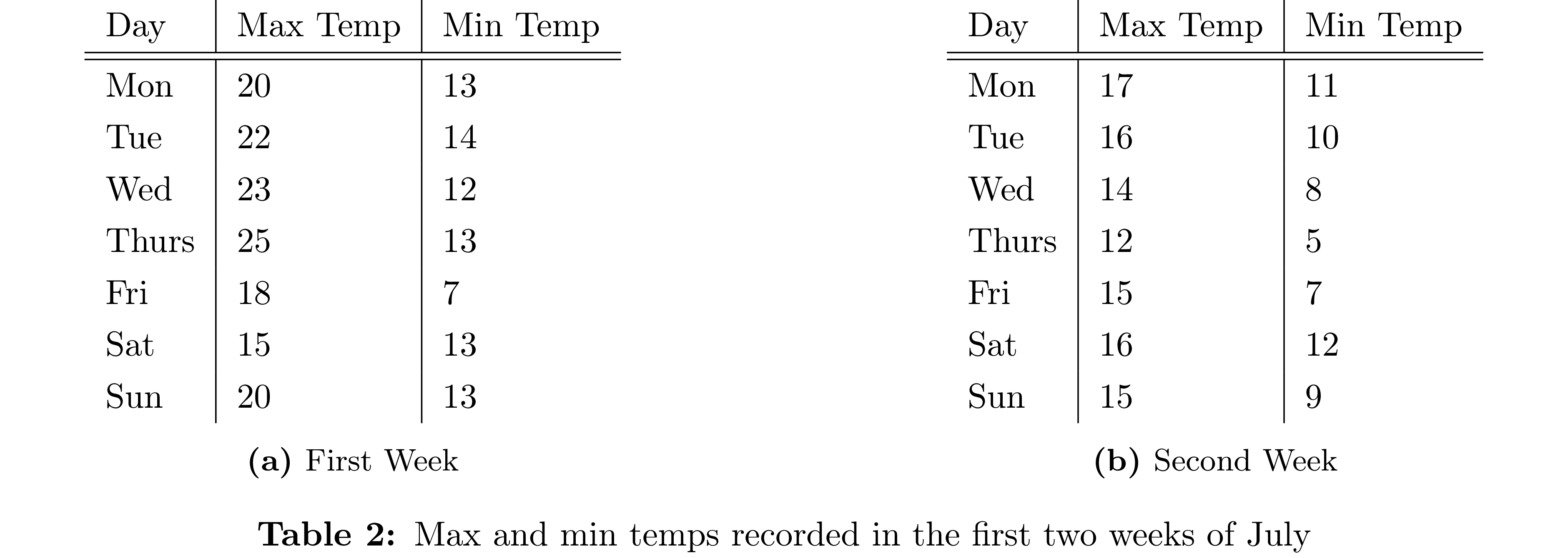
\caption{First Week}
\label{tab:week1}
\end{subtable}
\hfill
\begin{subtable}[h]{0.45\textwidth}
\centering
\begin{tabular}{l | l | l}
Day & Max Temp & Min Temp \\
\hline \hline
Mon & 17 & 11\\
Tue & 16 & 10\\
Wed & 14 & 8\\
Thurs & 12 & 5\\
Fri & 15 & 7\\
Sat & 16 & 12\\
Sun & 15 & 9
\end{tabular}
\caption{Second Week}
\label{tab:week2}
\end{subtable}
\caption{Max and min temps recorded in the first two weeks of July}
\label{tab:temps}
\end{table}
Multi-row/column table
We may stack multiple rows (with multirow) or columns together. This can also be used to change the alignment of a specific cell. For example:
\begin{tabular}{|l|l|l|l|}\hline
  \multirow{10}{*}{numeric literals} & \multirow{5}{*}{integers} & in decimal & \verb|8743| \\ \cline{3-4}
  & & \multirow{2}{*}{in octal} & \verb|0o7464| \\ \cline{4-4}
  & & & \verb|0O103| \\ \cline{3-4}
  & & \multirow{2}{*}{in hexadecimal} & \verb|0x5A0FF| \\ \cline{4-4}
  & & & \verb|0xE0F2| \\ \cline{2-4}
  & \multirow{5}{*}{fractionals} & \multirow{5}{*}{in decimal} & \verb|140.58| \\ \cline{4-4}
  & & & \verb|8.04e7| \\ \cline{4-4}
  & & & \verb|0.347E+12| \\ \cline{4-4}
  & & & \verb|5.47E-12| \\ \cline{4-4}
  & & & \verb|47e22| \\ \cline{1-4}
  \multicolumn{3}{|l|}{\multirow{3}{*}{char literals}} & \verb|'H'| \\ \cline{4-4}
  \multicolumn{3}{|l|}{} & \verb|'\n'| \\ \cline{4-4}          %% here
  \multicolumn{3}{|l|}{} & \verb|'\x65'| \\ \cline{1-4}        %% here
  \multicolumn{3}{|l|}{\multirow{2}{*}{string literals}} & \verb|"bom dia"| \\ \cline{4-4}
  \multicolumn{3}{|l|}{} & \verb|"ouro preto\nmg"| \\ \cline{1-4}          %% here
\end{tabular}
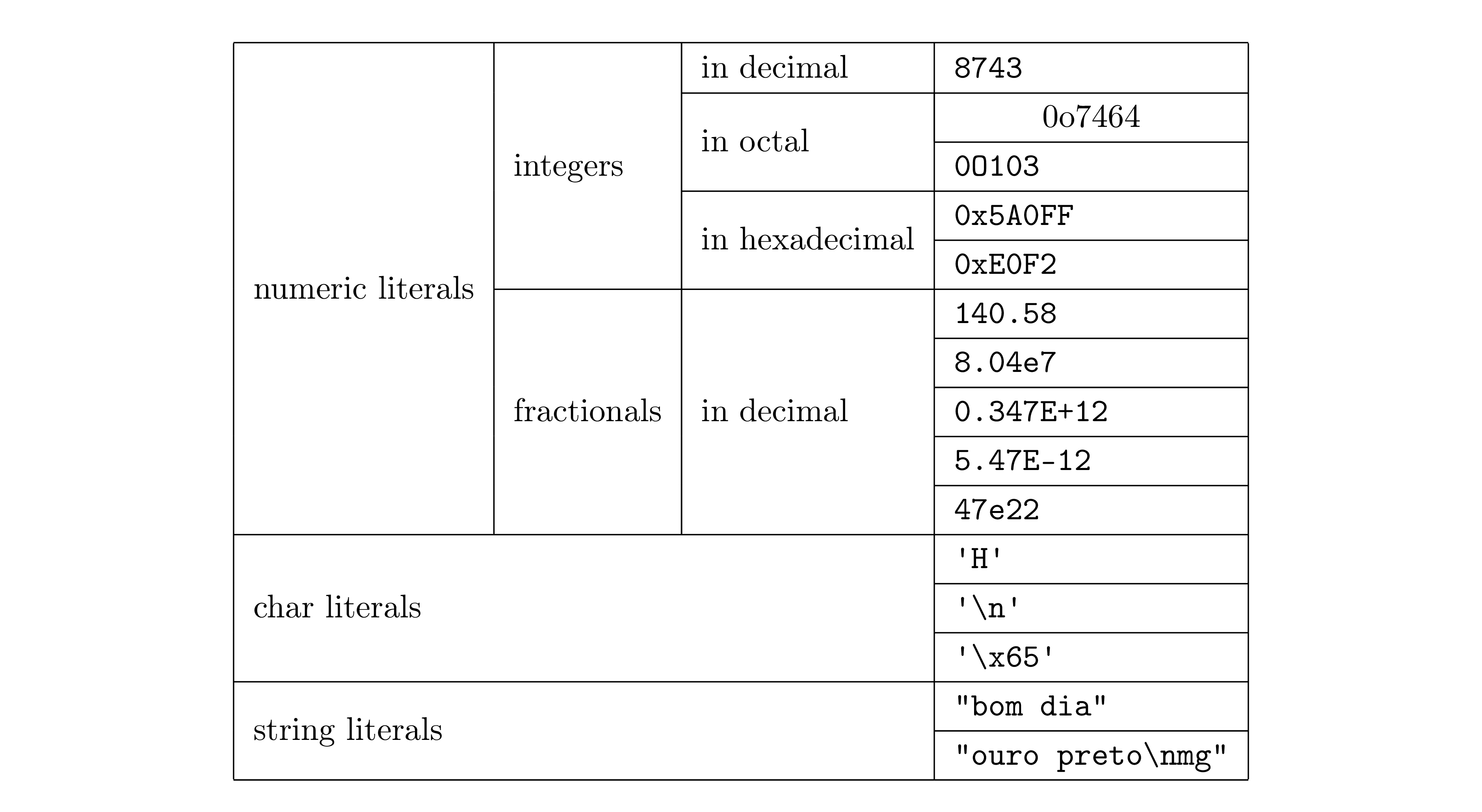
Note that, by default, the vertical boarders in a \multicolumn{}{}{} is ignored, so must be specified if wanted.
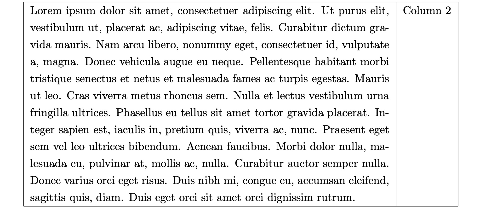
Wrapping text in a column
Specify a fixed-width column (p{…}) to get automatic line-breaks:
\begin{tabular}{ | p{0.7\linewidth} | l | }
\hline
\lipsum[1] & Column 2 \\
\hline
\end{tabular}
Long tables
For tables spanning pages, use longtable with customizable headers/footers:
\begin{longtable}{|c|c|c|}
\hline
% Common header for all pages
\textbf{Column 1} & \textbf{Column 2} & \textbf{Column 3} \\
\hline
\endfirsthead
% Continued header for subsequent pages
\hline
\textbf{Column 1} & \textbf{Column 2} & \textbf{Column 3} \\
\hline
\endhead
% Footer for intermediate pages
\hline
\multicolumn{3}{r}{\textit{Continued on next page...}} \\
\endfoot
% Footer for last page
\hline
\multicolumn{3}{c}{\textit{End of table}} \\
\endlastfoot
% Table content
1 & A & Alpha \\
2 & B & Beta \\
...
\end{longtable}
Equations
Load amsfonts,amsmath,amssymb for all documents with math. For (un)numbered equation blocks, use the align environment without math mode. For example:
\begin{align*}
x&=y           &  w &=z              &  a&=b+c\\
2x&=-y         &  3w&=\tfrac12 z    &  a&=b\\
-4 + 5x&=2+y   &  w+2&=-1+w          &  ab&=cb
\end{align*}
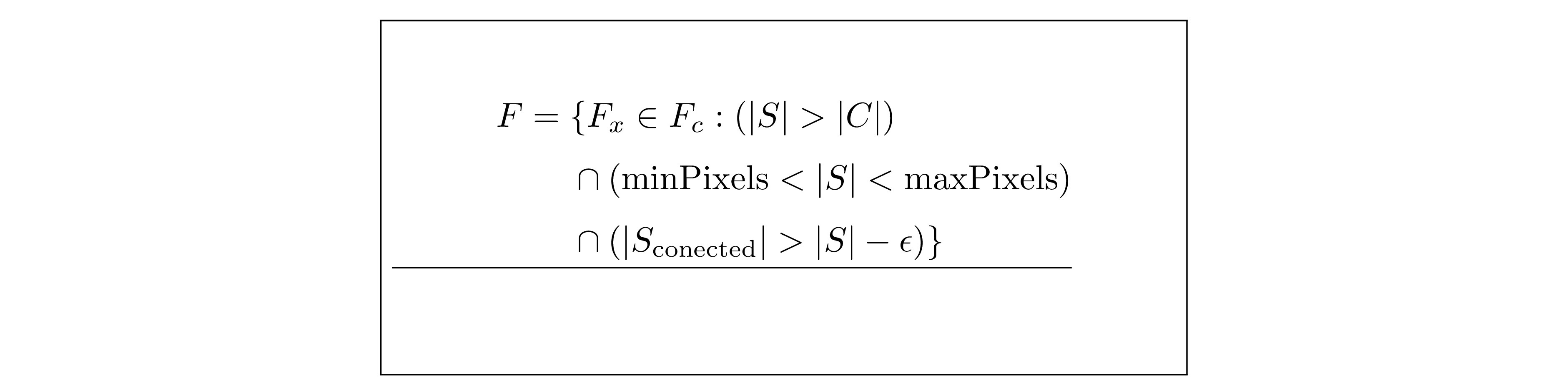
For a long, broken‐up equation:
\begin{align*}
F = & \{F_{x}\in F_{c}: |S|>|C|\\
      &\quad\cap (\minPixels<|S|<\maxPixels)\\
      &\quad\cap(|S_{\mathrm{connected}}|>|S|-\epsilon)\}
\end{align*}

Note that any operators of the RHS should align with the right of the (in)equality sign. Also, do not put \\ in blocks unless a new line is needed, otherwise extra space would be created:
Sometimes you may want to name a equation instead of numbering it, use \tag{} is this case:
\begin{equation}
Y = \alpha + \beta X^\top + \varepsilon \tag{Baseline} \label{eq:baseline}
\end{equation}

Note your math should end with punctuation if you want to embed it in a sentence.
Theorems and Definitions
Use amsthm for theorems, definitions, remarks, etc. Define environments in the preamble:
\newtheorem{theorem}{Theorem}
\theoremstyle{remark}
\newtheorem*{remark}{Remark}
\theoremstyle{definition}
\newtheorem{definition}{Definition}
There are three styles of blocks available, plain, definition, and remark. To number according to sections, chapters or theorem (for corollaries), add [anchor] at the end of the definition in the preamble. For example, adding \newtheorem{corollary}{Corollary}[theorem] produces Corollary 1.1.
For a box wrapping the block, use mdframed. Wrap the block by the mdframed environment for a local change. To wrap all the blocks, put the following in the preamble:
\surroundwithmdframed{theorem}
\surroundwithmdframed{definition}
\surroundwithmdframed{remark}
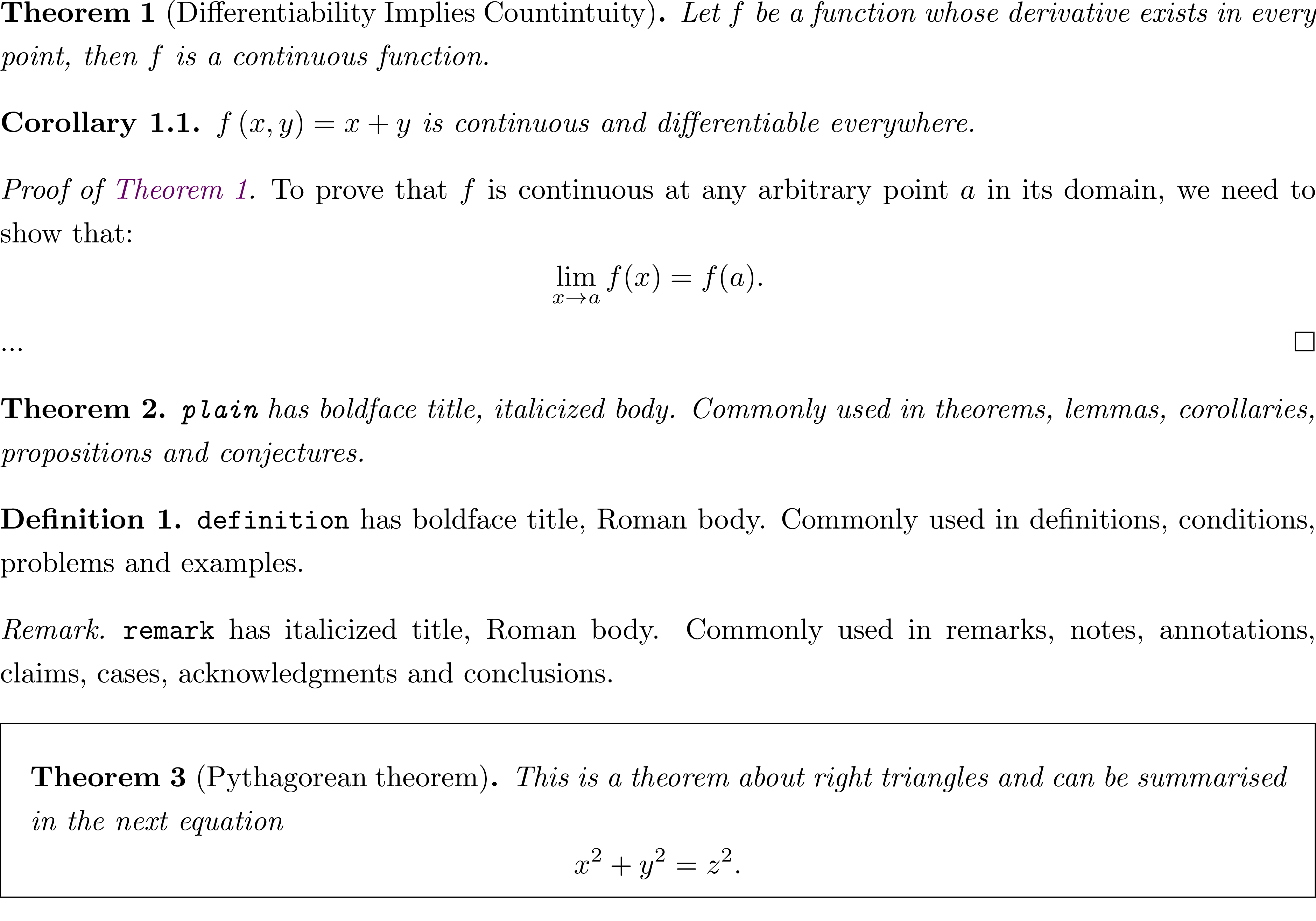
Then the following code
\begin{theorem}[Differentiability Implies Countintuity] \label{thm:diff}
Let \(f\) be a function whose derivative exists in every point, then \(f\) is a continuous function.
\end{theorem}

\begin{corollary}
\(f\left(x,y\right)=x+y\) is continuous and differentiable everywhere.
\end{corollary}

\begin{proof}[Proof of \autoref{thm:diff}]
To prove that \( f \) is continuous at any arbitrary point \( a \) in its domain, we need to show that:
\[
\lim_{x \to a} f(x) = f(a).
\]

...
\end{proof}

\begin{theorem}
\mintinline{latex}{plain} has boldface title, italicized body.
Commonly used in theorems, lemmas, corollaries, propositions and conjectures.
\end{theorem}

\begin{definition}
\mintinline{latex}{definition} has boldface title, Roman body.
Commonly used in definitions, conditions, problems and examples.
\end{definition}

\begin{remark}
\mintinline{latex}{remark} has italicized title, Roman body.
Commonly used in remarks, notes, annotations, claims, cases, acknowledgments and conclusions.
\end{remark}

\begin{mdframed}
\begin{theorem}[Pythagorean theorem]
\label{pythagorean}
This is a theorem about right triangles and can be summarised in the next
equation
\[ x^2 + y^2 = z^2. \]
\end{theorem}
\end{mdframed}
would produce
Code
-
Inline code: use backticks:
\verb|…|or\mintinline{python}{…} -
Display code (no highlighting):
\begin{verbatim}
from sklearn.neural_network import MLPClassifier
\end{verbatim}
gives
from sklearn.neural_network import MLPClassifier -
With
minted(syntax-highlighted):\begin{minted}{latex} from sklearn.neural_network import MLPClassifier \end{minted}gives
from sklearn.neural_network import MLPClassifier
Note that inline code snippets are non-breakable. To caption a minted block, wrap it in a listing float just like figures/tables.
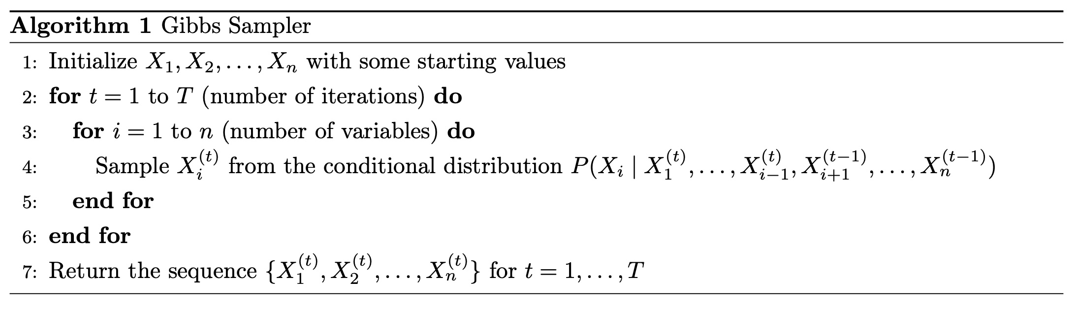
Algorithms
Use the algorithm + algorithmic packages:
\begin{algorithm}[htbp]
\caption{Gibbs Sampler}
\label{alg:gibbs}
\begin{algorithmic}[1]
  \STATE Initialize $X_1,\dots,X_n$.
  \FOR{$t=1$ to $T$}
    \FOR{$i=1$ to $n$}
      \STATE Sample $X_i^{(t)}\sim P(X_i\mid X_{-i})$.
    \ENDFOR
  \ENDFOR
  \STATE Return $\{X^{(t)}\}_{t=1}^T$.
\end{algorithmic}
\end{algorithm}
Layout
- Quotation marks: use `` and
''. -
Margins: To adjust margins and paper size, use the following code in the preamble:
\usepackage{geometry} \geometry{a4paper, margin=1in} - Fonts: It is recommended to use pdfTeX. Use
newtxtext/newtxmathfor Times,newpxtext/newpxmathfor Palatino. - Font size: Document-level:
\documentclass[12pt]{article}; local:{\small …}etc.: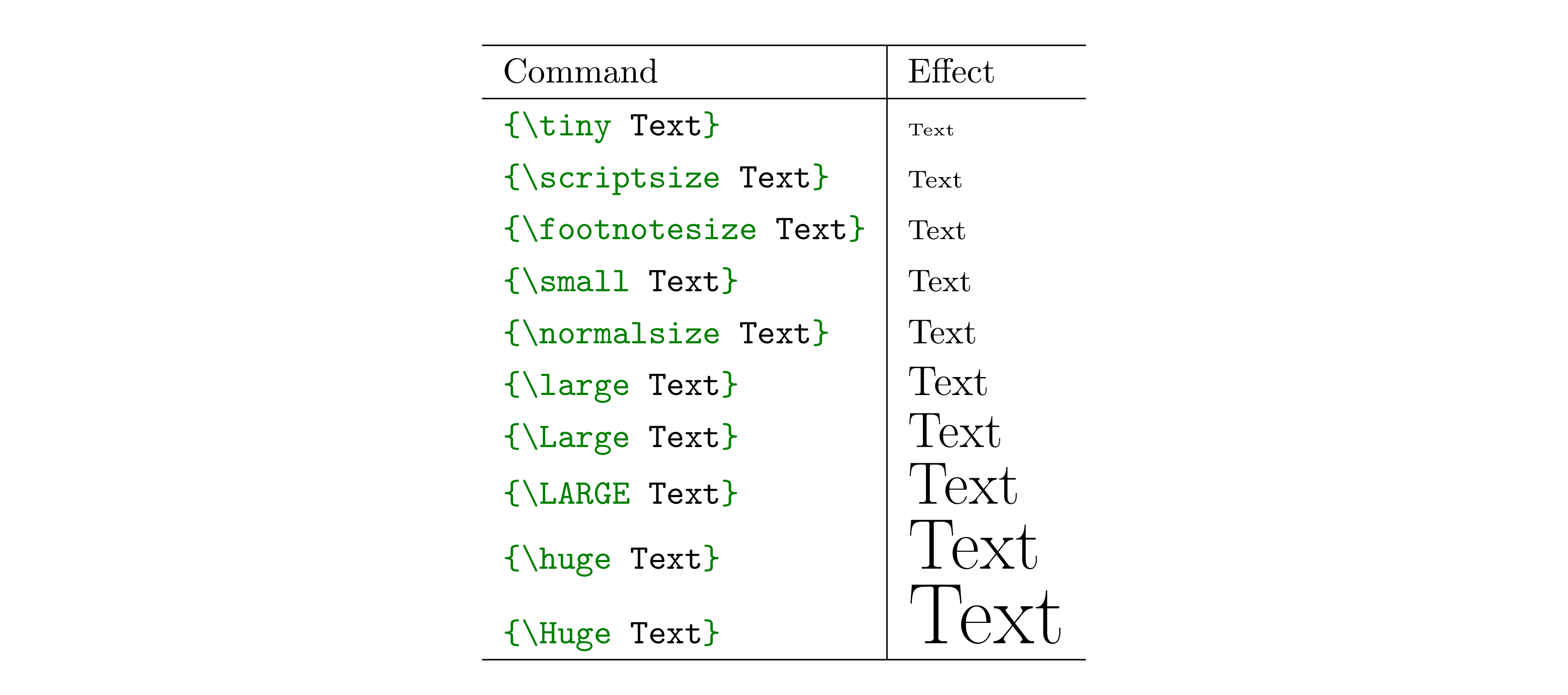
-
Hyperlinks: To use hyperlinks, use
hyperreffor general links andurlfor URLs. To customize colors, do something like:\usepackage{hyperref} \usepackage[dvipsnames]{xcolor} \usepackage{hyperref} \definecolor{DarkNavy}{rgb}{0.0, 0.0, 0.5} \definecolor{DeepMaroon}{rgb}{0.5, 0.0, 0.0} \hypersetup{ colorlinks = true, linkcolor = DarkNavy, % for \ref and internal links citecolor = DeepMaroon, % for \cite urlcolor = DarkNavy, % for external URLs filecolor = OliveGreen % for local file links }Use
\autoref{…}and\nameref{…}for links. For example, referring back to the images in Figures,\autoref{fig:1-image}and\autoref{fig:2-image-a}would produceFigure 1 and Figure 2a. Use meaningful labels with prefix (for example, the label forAlgorithm 1is\label{alg:gibbs}) so that it would be easy to recall them. However, for some floats, such as algorithm boxes, the name for references might not be predefined. In these cases, use the command\newcommand{\algorithmautorefname}{Algorithm}to define them. If it is already defined but needs to be changed (say, capitalizing), use\renewcommand{\algorithmautorefname}{Algorithm}. To refer directly to the name of the section or the caption of the float, use, for example,\nameref{sec:figure}and\nameref{alg:gibbs}forFigures and Gibbs Sampler. This works for math similarly,\autoref{eq:baseline}producesEquation Baseline. It also works for theorems. - Line spacing: Use
\onehalfspacing(viasetspacepackage). Note that this does not change spaces in other environments, such as captions. However, note that this means that the original space between lines are multiplied by 1.5. This is different from Microsoft Word or Apple Pages, which set the space between lines as 1.5 times the vertical space of texts. - Paragraph spacing: Load
parskipto disable indentations and use spacing to distinguish paragraphs. - Indentations: Disable locally with
\noindent, or loadindentfirstto indent first paragraphs. - Forced spaces: In some cases, spaces are ignored after a command, use
~to force it, e.g.\LaTeX~document. - Vertical space: Use
\vspace{…}but it automatically halts at the beginning/end of a page, use\vspace*{…}to force it. -
Accented letters: To use accented letters directly (copying and pasting), load
\usepackage[utf8]{inputenc} % usually not needed (loaded by default) \usepackage[T1]{fontenc} -
Landscape pages:
\usepackage{pdflscape}
…
\clearpage
\begin{landscape}
  …
\end{landscape}
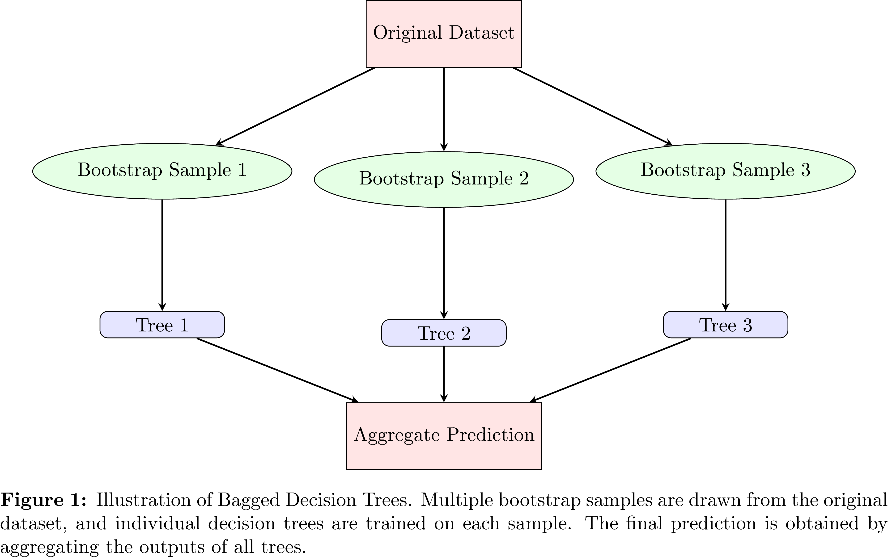
TikZ
Using TikZ for illustration makes the content clear and consistent. Use PowerPoint/Keynotes/Google Slides to make your life easier.
\begin{figure}[htbp]
    \centering
    \begin{tikzpicture}[
        tree/.style={rectangle, draw, fill=blue!10, text width=2cm, text centered, rounded corners},
        bootstrap/.style={ellipse, draw, fill=green!10, minimum height=1cm, text centered},
        box/.style={rectangle, draw, minimum width=1.5cm, minimum height=1.2cm, fill=red!10},
        arrow/.style={thick,->,>=stealth}
    ]

    % Original Dataset
    \node[box] (data) {Original Dataset};

    % Bootstrap Samples
    \node[bootstrap, below left=1.5cm and 2cm of data] (sample1) {Bootstrap Sample 1};
    \node[bootstrap, below=1.5cm of data] (sample2) {Bootstrap Sample 2};
    \node[bootstrap, below right=1.5cm and 2cm of data] (sample3) {Bootstrap Sample 3};

    % Decision Trees
    \node[tree, below=2cm of sample1] (tree1) {Tree 1};
    \node[tree, below=2cm of sample2] (tree2) {Tree 2};
    \node[tree, below=2cm of sample3] (tree3) {Tree 3};

    % Aggregation
    \node[box, below=1cm of tree2] (aggregate) {Aggregate Prediction};

    % Connections
    \draw[arrow] (data) -- (sample1);
    \draw[arrow] (data) -- (sample2);
    \draw[arrow] (data) -- (sample3);

    \draw[arrow] (sample1) -- (tree1);
    \draw[arrow] (sample2) -- (tree2);
    \draw[arrow] (sample3) -- (tree3);

    \draw[arrow] (tree1) -- (aggregate);
    \draw[arrow] (tree2) -- (aggregate);
    \draw[arrow] (tree3) -- (aggregate);

    \end{tikzpicture}
    \caption{Illustration of Bagged Decision Trees.
    Multiple bootstrap samples are drawn from the original dataset,
    and individual decision trees are trained on each sample.
    The final prediction is obtained by aggregating the outputs of all trees.}
    \label{fig:bagged_decision_trees}
\end{figure}